PWM/PID Motor Control using Orangutan from Pololu:

Hardware and Software Tests

Jim Remington

This site was created to share some experiences with the nice little Orangutan controller from Pololu corp. The Pololu folks are great engineers but despite enthusiastic promises of examples to come, they do not seem to be able to provide software support for their products. They need help from their users! I'll be happy to post code/links/comments from others here. For example, Cathy Saxton of Idle Loop Software Design has posted an extensive C++ code example for the Orangutan that is well worth studying. Here, I provide some vanilla C examples.

The Orangutan is based on the ATmega8 controller from Atmel, which is great because of the availability of excellent free development software -- especially WinAVR. I use PIC processors when I can because the instruction set and hardware is so simple, but usually program them with MPLAB in assembler. PIC C compilers are expensive, and not as flexible as the fine gcc compiler.

The down side is that the built-in hardware of the ATmega chips is extremely flexible and the documentation is very hard to read. So, just getting a simple pulse-width modulated motor controller working can be difficult hard unless you have examples to follow. Read on:

The development system

I use a laptop running WinXP Pro connected to the AVRISP programmer via a USB serial cable adapter. The USB serial port ends up being different COMn ports depending on which USB port it is plugged in to, so the makefile often has to be edited. The makefile that I'm currently using is here. I have the Atmel development software installed but I've only used it once for a medium-sized assembly language project. C is certainly less work, but quirky and less intimate.

Robot testbed

The test bed is a home-made minisumo rig controlled by the Orangutan. The motor controller drives two standard servos, modified for free rotation and from which the electronics have been removed. The entire thing is powered by a single 6 volt alkaline battery pack.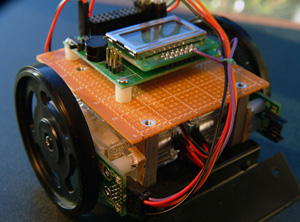

"WheelWatcher" modules (WW-01) from Nubotics, attached to the servo bodies, were used to measure the wheel rpms. The code examples provided by Nubotics were useful to figure out how to use the modules, but the examples are very complex--far more complex than they need to be to get the basic job done. I monitored only the right wheel in my tests. The clock output of the WW-01 (purple lead) was connected to INT0 (PORTD.2), which unfortunately is required as an output to the Orangutan LCD module. An INT0 interrupt routine counts segment ticks and measures the period of wheel rotation (time between segment ticks), accumulating average values. The direction of wheel rotation and total travel distance was monitored by the same routine, with the WW-01 direction bit (orange wire) connected to PORTC.5. The distance and direction information were not used in my example, but could be used for dead reckoning. This setup was later used to implement error-correcting proportional (PID) speed control, as PWM alone is insufficient for robust speed control. See below.

My opinion of the WheelWatcher? Glad you asked! A good idea, but too expensive and too limited in mounting flexibility for different motor/wheel configurations--I now have a spare set that won't fit my other applications. Also, if you make a mistake applying the black-and-silver reflective wheel sticker, the replacement cost is outrageous -- $5.00 plus shipping at one supplier.

The wheel speed is measured by computing the period between segment ticks. Timer0 increments at 3.9 kHz and when it overflows, an interrupt causes a counter to be incremented, extending the resolution to 24 bits. As each wheel tick occurs, a time stamp is saved and used to compute the period after the next tick. This approach fails when the wheel is stalled, so a more complete routine (see PID code below) should include a timeout to indicate zero velocity.

The LCD display on the Orangutan is good for accumulating the information on the wheel rotational period as a function of the PWM setting, but care has to be taken to disable the INT0 interrupt and reinitialize the LCD output bit on PORTD, as they can't be used by the two routines simultaneously. The actual test code, not cleaned up for publication, is WW_pwm_test.c, which requires routines to run the LCD display lcd_or.c (modified from an example posted on the Polulo user forum) and one of the PWM modules mentioned below. This program steps through a series of PWM settings, measures the wheel rotational period, and outputs the period and PWM setting on lines 1 and 2 of the LCD display, respectively. The wheel speed is calculated in arbitrary units as 1/(period*0.256E-3)--see graphs below.

On board motor controller

The on-board LB1836M dual H-bridge has four modes of operation (taken from the data sheet, available from Pololu, or here.)

IN1/3 IN2/4 OUT1/3 OUT2/4 Mode

H L H L Forward

L H L H Reverse

H H L L Brake

L L Off Off Coast

Forward and reverse modes are obvious, however the difference between the "brake" and "coast" or output-off modes is less obvious. Brake mode is in principle supposed to stop the motor quickly by acting as a short circuit across the motor terminals, but the current must flow through one of the output surge suppressor diodes as well as an output transistor, depending on the direction of motor rotation. The forward voltage drop across these components limits the effectiveness of the braking action Conversely, in "output off" mode the outputs do not conduct current and the motor coasts or freewheels. Either mode can be used for PWM control but the results are quite different (see below).

Brake action is power hungry

In brake mode, in order to hold the outputs low at the rated collector current, base current must flow in the output transistors. I measured this to be about 30 mA for each bridge (which is in agreement with the chip documentation), so about 60 mA is wasted to hold the outputs low if the motors are not rotating. A controller with FET output transistors may be a better choice, but according to fearless leader ;) Don Rumsfeld, you go to war with what you have. To save power, the motor outputs should be turned off any time braking action is not needed. I have not implemented this in my code, except for the case that speed=0.

PWM modes

The Timer1 module of the ATmega8 provides several PWM modes. I experimented with two of these: 8-bit phase correct PWM (mode 1) and 8-bit fast PWM (mode 5). There is no need to use more than 8 bits of speed resolution. NOTE that the timer/counter1 registers are 16 bits wide, so in 8-bit PWM modes, take care to avoid setting speeds > +/- 255 or unexpected results will occur. In either mode, timer/counter register TCNT1 increments at a set rate and the value is continuously compared to the contents of registers OCR1A and OCR1B. When a match is reached, the bit OC1A or OC1B is set or cleared according to the setting of the TCCR1A control register and this action can cause a port bit, e.g. PB.1 or PB.2 to be set or cleared. In turn, PB.1, PB.2 and PD.5, PD.6 set the state of the LB1836M motor controller, according to the above table. To avoid confusion, in the code I've followed the LB1836M documentation with regard to the definition of "forward" and "reverse", but simply reversing the motor leads reverses these. There is actually a good reason to do so, given the design of the Orangutan. This is because the motor off-state during the PWM cycle can be either braking or coasting, depending on the controller configuration, and the two states do behave differently.

8-bit Phase Correct Mode

This mode is easy to use and does not require interrupt programming. According to the ATmega8 documentation, this mode is preferred for motor control, but I didn't see a difference compared to fast PWM mode except for cycle time. In my implementation (see code pwm_8PC_direct.c), for forward motion, OC1A=PB.1 is set high as TCNT1 increments, until match is reached with OCR1A and then it is set low (likewise for PB.2). After TCNT1 reaches 255 (0xFF), it reverses direction and counts down until a match is again reached, and PB.1 (PB.2) is set high again. Thus, the right motor is ON until TCNT1=OCR1A and then it is off until TCNT1 counts down again to rematch, whereupon it is turned on again, ad infinitum. The direction of travel (and the nature of the "off" state) depends on the setting of PORTD bits 5 and 6. In my code, forward motion alternates with "coast" and reverse motion alternates with "brake" but this could be changed by swapping motor leads and the speed variables. Forward PWM does not have the same relation between speed and PWM (OCR1A/B) setting or motor current draw as does reverse PWM, see below.

8-bit fast PWM

In this mode, TCNT1 counts from 0 to 0xFF and then overflows to 0. If desired, an interrupt is generated when this overflow occurs. As in other modes, TNCT1 is compared to OCR1A and OCR1B, and the bits OC1A and OC1B are set or cleared on match. This can be used to provide PWM without interrupts as in the above case, that is, PORTB bits 1 and 2 can be made to change accordingly by the hardware. However, as in the previous example, forward and reverse "off" modes are different. In order to get around this, the bits OC1A and OC1B must be disconnected from PORTB and the appropriate actions are then taken by interrupt routines. In my implementation, when TCNT1 overflows, the motors are turned on in the appropriate direction, as determined by the global variables r_speed and l_speed. When TCNT1 matches OCR1A or OCR1B, the right or left motor is turned off, either in brake mode or coast mode, depending on which code example is loaded. A special case occurs when l_speed or r_speed=0, in which case the motor is never turned on. This avoids glitches in the output.

In my implementation, three interrupt service routines are required (TCNT1 Overflow, Compare matches TCNT1=OC1A and TCNT1=OC1B). The basic routines pwm_brake.c and pwm_coast.c were written to implement this approach and to study current draw and wheel rotational period (converted into robot forward speed) as a function of the PWM settings. Hopefully this example will be useful to others. Please feel free to offer corrections or suggestions. The example driver program pwm_modetest.c can be used to call one of the two PWM routines and exercise the motors.

If the foregoing is not completely clear, well, there is always the ATmega8 chip documentation...

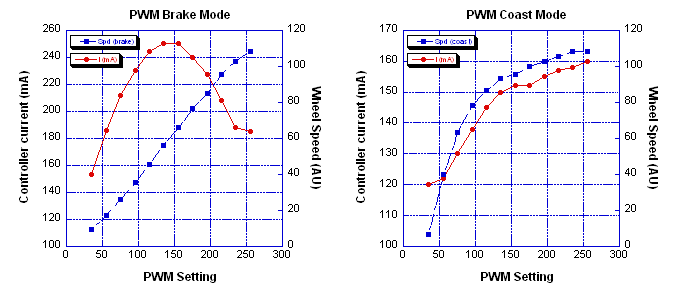
PWM mode tests

Although 255 motor speed steps are permitted, the gears are stiff enough that even when held off the ground, the wheels on my test rig don't rotate until the PWM setting is about 35, and little difference is seen for increments of 1 step. I chose to monitor free rotation of the robot wheel, that is, the robot did not need to drag itself around. Needless to say the LCD display is hard to read when moving! Besides, everyone's robot will behave differently.

I measured the overall current draw of the entire robot (Orangutan plus motor controller plus WheelWatcher) by a multimeter in series with the battery leads. With the motors off in "coast mode" about 60 mA was consumed. With motors off in "brake mode" about 120 mA was consumed, due to ~60 mA base current for the output transistors in the motor driver chip. Maximum current draw for "free air" rotation (right wheel only) was around 250 mA in brake mode PWM. The current draw is of course higher if the robot is running on the ground.

For brake mode, the wheel speed is very linear with the PWM setting but the current consumption is generally high and very nonlinear with the PWM setting. Graphs of the results are posted below. As you can see, the current draw is highest when the motor is running at about half speed. This makes perfect sense: for half of the PWM cycle, the rotational energy is being dissipated by the braking action. However, the speed setting is quite robust, that is, low speed performance is good, and the robot maintains its speed rather well if a bit of resistance is applied to the wheel. Why this should be so is less obvious, and it is not true for coast mode. .

For coast mode, the wheel speed is a nonlinear function of the PWM setting, and tops out at well below PWM setting=255. The current draw at low to intermediate speeds is quite a bit lower than with brake mode, but about the same when both are maxed. However, at intermediate speeds, the wheel rotational rate is not robust and slight resistance applied to the wheel causes it to slow down rather quickly. In the graphs at right, wheel speed is in arbitrary units (AU).

Note on CPU clock speeds

The Orangutan is shipped with the default CPU clock speed of 1 MHz. At best this leads to a PWM cycle time of 3.9 kHz for 8 bit resolution. Higher frequencies of 10-20 kHz are said to be advantageous. You can reprogram the ATmega8 fuses to use an 8 MHz internal clock, which I did using AVR Studio 3.56 (when selecting the device programmer, a window opens allowing you to change fuse settings). All of the examples shown here work, given appropriate changes to the delay loops. The power drain and speed tests described above are reported for 1 MHz cpu clock only.

Preliminary conclusions: brake versus coast mode

For simple PWM speed control, brake mode has better linearity of speed versus PWM setting and speed is maintained reasonably well with changes in wheel motion resistance. However, current draw is high. With coast mode, current draw is much lower at intermediate speeds, but the speed is a nonlinear function of the PWM setting. Also, the speed depends strongly on resistance to wheel motion. However, if the speed is actively controlled by a PID algorithm, "coast mode" should be superior as the power draw is lower.

PID code

With the above code in place, it proved straightforward to implement a PD (Proportional/Derivative) algorithm to control the wheel rotational speed in the arbitrary range of [80,255]--at lower than 1/3 power, motor operation was found to be unreliable. "Coast mode" PWM was used to save power. Wheel rotation is monitored by the WheelWatcher modules, although the only signal actually used is the segment tick. It would be much cheaper to use a phototransistor to peer through spokes or holes to get that signal. The basic program operation is as follows:

Main program posts speed request and sets an approximate PWM setting via the function call set_speed(left, right)
Ticks from WheelWatcher activate an interrupt that measures the current period, converts to velocity and applies the PD algorithm.
The PWM module is controlled by the PD algorithm, which modulates the motor power.
A Timer0 interrupt provides a basic clock tick that, among other tasks, counts down a separate timer for each wheel to detect a stall. If this happens, the PWM on time for that wheel is bumped up.

The algorithm is proportional/differential (PD) with an additional low-pass filter. I found it was not necessary to include an integral term.

Wheel rotational period is determined from the WheelWatcher ticks.
Period is low-pass filtered via per = 0.25*per + 0.75*last_per
speed = constant/per. Constant is chosen so that max speed=255
error = (requested_speed - current_speed)
delta PWM = Kp*error + Kd*(error - last_error).

The PD code

Works great! Take a look at the all-in-one example pid_kd_all.c.

Tuning the code

Tuning means to determine the mysterious constants Kp and Kd, which in turn will depend on the system: motor gear ratio, battery voltage, overall weight, friction, phase of moon, etc. There are entire web sites (plus thick, four-color, expensive, dense & excruciatingly boring undergraduate engineering texts) devoted to the process. Sadly, no standard notation seems to have arisen, not even the sign of the error term seems to be standard! It is easiest to start with floating point calculations and then convert to integer math for speed. You will probably need 8 MHz CPU clock or higher.

The basic operation of tuning is fairly simple: you begin with small Kp and Kd=0, and increase Kp until first the system response (e.g. motor speed) stabilizes, then further increase Kp until the response starts to oscillate. Back off Kp a bit, then, increase Kd in order to damp down the oscillations. In theory, there should at most one overshoot in response to a step change in speed.

For more detail, one place to start is the WikiPedia entry. However, Parallax Inc. has a great example of PID process control using the Basic Stamp. Finally, there is always Jeff Bachiochi's lovely example of magnetic levitation in Circuit Cellar (Issue 18, Dec-Jan 90-91), in which only 15 lines of BASIC code were required to levitate a steel sphere with an electromagnet. For another amusing example, see the PID-Pong levitating ping-pong ball challenge by Tom Cantrell in issue #50 of the same publication.

To facilitate tuning, you should have a means of studying the operation of the algorithm at fairly high speed. Following an example C program posted by Nubotics, I used high speed RS232 output (38400 baud) using the built-in UART to capture the action of the PD algorithm at 0.1 second intervals on a PC. All that is needed is a time stamp, the current speed and PWM settings, which is all the main loop of the test program does after posting a requested speed. The output was captured by HyperTerm and loaded into a spreadsheet for plotting. I found that the values for Kp and Kd were not critical, with Kp in the range of 0.1 to 0.2 while Kd needed to be about 0.4 to 0.6. 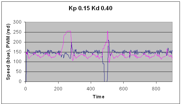After an evening of experimentation, I settled on Kp=0.15 and Kd=0.40. 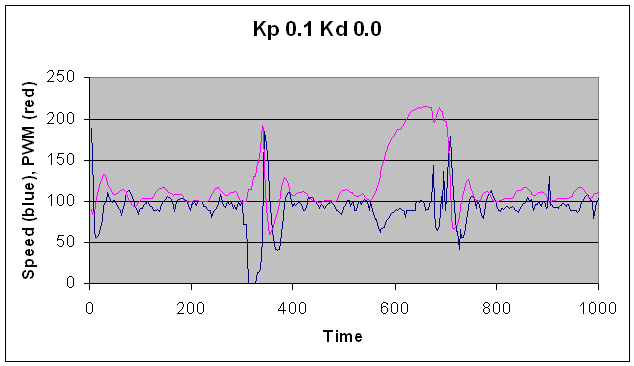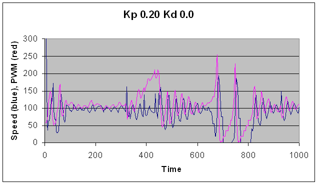See the plots below for some examples, with comments.

The graphs below show the speed and PWM setting for about 30 seconds. The horizontal axis is clock ticks.

Note:I physically grabbed the wheel at two points during each test (for a few seconds) to slow it down or stop it, so that I could observe the response.

Kp=0.1, Kd=0.0, note drift of speed about setpoint--too little feedback

Kp=0.20, Kd=0.0, note violent oscillation of speed about setpoint, too much feedback

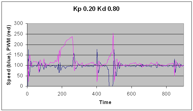
Kp=0.20, Kd=0.80. The violent oscillations are mostly damped by the error term, but the response is still jerky with large overshoots

Kp=0.15, Kd=0.40. Good enough--one overshoot is fine! (The regular oscillations in speed are due to slightly sticky gears)

RS232 interface

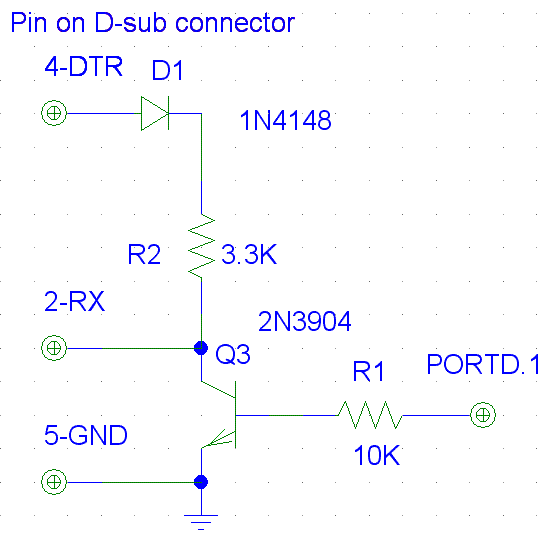
The RS232 AVR to PC transmit-only interface is port-powered from the PC DTR, pin 4 (or RTS, pin 7) and it worked well at 38400 baud using a USB to serial adapter. Similar designs can be found in many places on the web, see for example the PICList site. A schematic diagram is available here. The diode is probably necessary as on my adapter, the RTS and DTR pins swing from about +8V when the port is open to -8V when the port is closed, which could damage the transistor. 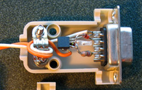I built the circuitry into a D9 subminiature shell as shown above.

Feel free to email me with comments, questions or suggestions.
last update: 10/1/2006

IN1/3	IN2/4	OUT1/3	OUT2/4	Mode
H	L	H	L	Forward
L	H	L	H	Reverse
H	H	L	L	Brake
L	L	Off	Off	Coast