 Molecular Dynamics -
Integration Errors Molecular Dynamics -
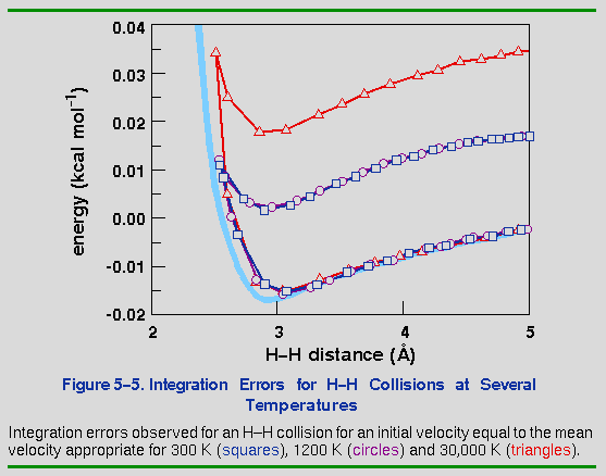
Integration Errors
Molecular Dynamics -
Integration Errors Molecular Dynamics -
Integration Errors
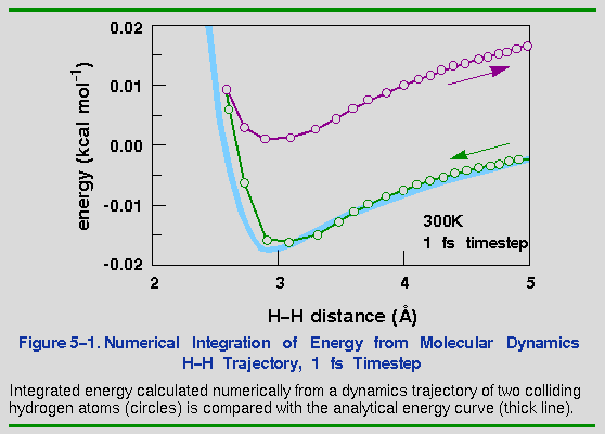
To illustrate this, consider the collision of two atoms. Figure 5-1 plots the true potential energy of the van der Waals potential between two hydrogens along with the energy integrated numerically from the forces. The time step used is 1 fs at a temperature of 300 K. The temperature is set by assigning an initial velocity of 1500 m s-1 (0.015 Å fs-1) to one of the hydrogens along the vector connecting them. This velocity is the most probable velocity of a hydrogen atom at 300 K.
As the two atoms approach each other, the integration agrees well with the analytic curve. However, after the atoms collide, the integrated energy is significantly higher than the true energy. This behavior is due to the atom moving too quickly through a rapidly changing energy function. When the atoms are far apart, the energy change is smallest and therefore, the forces are smallest and most linear. As the atoms approach, they speed up and take larger and larger steps, until they reach their highest velocity at the energy minimum. Unfortunately, this is precisely where the forces start changing the fastest. Thus, when the atoms should be taking large steps (far apart), they are taking the smallest steps, and when they should take small steps (near the minimum), they take the largest steps. The consequence is that the particles "step through" the energy barrier momentarily. Of course, once a new force is calculated at the extrapolated coordinate, the trajectory is rapidly corrected. However, it is too late for the energy integral-some energy has been gained.
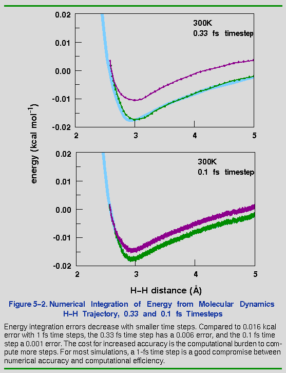
In this example, the total energy rose by about 0.02 kcal mol-1. Whether this is a reasonable error depends on how closely the exact motions need to be reproduced. Figure 5-2 shows the same curve as Figure 5-1, but with timesteps of 0.33 and 0.10 fs. Both give better results than 1.0 fs, but it is not clear whether the extra time required to calculate the smaller timesteps is worthwhile.
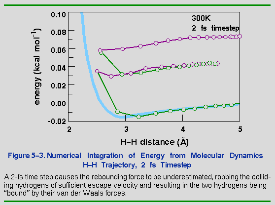
The consequences of too large a time step are much more dramatic. Doubling the time step from 1 to 2 fs results in an unusual artifact for the H-H system (Figure 5-3). In this case, the integration error not only affects the potential energy, but the kinetic energy as well. Momentum is removed, so that the hydrogens no longer have the velocity needed to escape after the collision. Of course, once momentum is lost, the atoms are trapped forever (barring an inverse error that could impart momentum). The atoms now vibrate back and forth (only 2 cycles are plotted in Figure 5-3), and each cycle incurs an additional integration error.
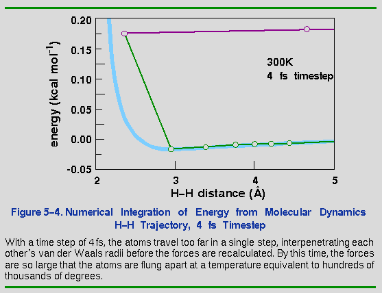
Increasing the time step another factor of 2 to 4 fs (Figure 5-4) finally causes the system to "blow up". The timestep is so long that the atoms deeply interpenetrate each other's steeply repulsive wall between steps. The resulting force is now so large that the atoms fly off at a speed of about 1 Å fs-1 (or 105 m s-1). An equivalent temperature would be in the hundreds of thousands of degrees.
To complete the analysis of integration errors, it is instructive to compare the effects of increasing kinetic energy on the stability of the numerical integration. Figure 5-5 shows that there is essentially no difference in the error between 300 and 1200 K. Going as high as 30,000 K only almost doubles the error, indicating that dynamics simulations are not as sensitive to the temperature as to the timestep.
 Main
access page
Main
access page  Theory/Methodology access.
 Dynamics access
 Dynamics - Choice of Timestep
 Dynamics - Stages & Duration of Runs
Copyright Biosym/MSI